Every quarter, companies that lobby the federal government file a form listing the people doing the lobbying. If one of those people used to work for a member of Congress or a federal agency, the filing has to say so. That disclosure is the "revolving door," and it is public.
The intuition is obvious. A lobbyist who spent six years as a senator's chief of staff gets meetings that a career K Street hand cannot. So a company that adds those people to its roster should get more out of every dollar it spends on lobbying, and if the market is slow to notice, its stock should do better than an equally heavy lobbyist without the connections.
This tutorial tests that idea six ways over nearly a decade. A static ranking by connections is the baseline. The change in connections is the core idea. Two blends pair that change with lobbying spend. One version restricts it to federal contractors. And a control portfolio of heavy lobbyists with no revolving-door hires at all sets the bar the thesis actually has to clear.
Everything here, including daily prices, comes from a single Quiver API key. There is no second data vendor to sign up for.
Getting Set Up with the Quiver API
This strategy needs three Washington datasets: who a company pays to lobby, which of those lobbyists used to work inside government, and what federal contracts the company wins. Assembling any one of them from the raw filings is a project in itself. The revolving-door disclosures alone are free-text "covered position" strings buried in quarterly filings, with no ticker attached.
Quiver has done the ticker mapping and the history for all three, and serves adjusted daily prices from the same API. That last part matters more than it sounds: a backtest usually means a second vendor, a second key and a second rate limit. Here one Hobbyist plan covers the whole pipeline.
1. Create an account and grab your API key
Every Quiver endpoint requires authentication. There is no anonymous tier of the data itself, so the first thing you need is a key. The key ties your requests to a rate limit and to the datasets your plan is entitled to.
This tutorial uses Corporate Lobbying, Government Contracts, the Revolving Door feed and Historical Daily Prices. All four are Tier 1 endpoints, which the Hobbyist plan covers. There is no reason to pay for Trader unless you plan to extend the strategy into insider trading, 13F holdings or patents.
Head to the Quiver API pricing page to create an account and pick a plan. The Hobbyist plan ($30/mo, or $25/mo billed annually) covers everything this tutorial needs. Use code 50YEAR at signup for 50% off your first year.
Install the dependencies and put the key in a .env file at the root of your project. The script reads it with django-environ so it never ends up hardcoded in source.
pip install requests pandas "plotly<6" vectorbt kaleido==0.2.1 django-environ

# .env in the project root -- never commit this file. One key is all you need.
quiver_api_key=your_quiver_key_here
2. Authentication and a first call
Quiver uses a bearer token: every request carries an Authorization: Bearer <key> header and nothing else. Confirm it with one cheap call before building anything on top of it. The revolving-door feed is a good first target because its field names are the ones the rest of the script depends on.
import environ, requests

env = environ.Env()
environ.Env.read_env(".env")

API_KEY = env("quiver_api_key")
BASE_URL = "https://api.quiverquant.com"
HEADERS = {"Authorization": f"Bearer {API_KEY}"}

# One cheap call to prove the key works before building anything on it.
resp = requests.get(f"{BASE_URL}/beta/live/revolvingdoor", headers=HEADERS, params={"page_size": 2})
resp.raise_for_status()
print(resp.json()[0].keys())
# dict_keys(['DatePosted', 'Ticker', 'Client', ..., 'LobbyistID', ..., 'CoveredPosition',
#            'Branch', 'Chamber', 'FormerEmployer', 'BioGuideID', 'NewLobbyist', ...])
3. Which endpoints, and how many calls
Lobbying, contracts and prices are per-ticker historical endpoints of the form /beta/historical/{dataset}/{ticker}. To cover the point-in-time S&P 500 you loop over 771 tickers, three times. The revolving-door feed is different: /beta/live/revolvingdoor takes date_from and date_to on the posting date and pages a thousand rows at a time, so one pass over the whole feed, about 135 pages back to January 2016, covers every company at once.
That is roughly 2,500 requests, and the Hobbyist rate limit will push back with 429 responses along the way. Every call therefore goes through a retry wrapper with exponential backoff that returns None when it gives up rather than raising, so one stubborn ticker cannot kill forty minutes of progress. It retries on 5xx as well as 429; Quiver's infrastructure occasionally returns a transient 500 and treating it as fatal throws away real work.
import time
import pandas as pd

def get_with_retry(url, params=None, max_retries=5):
    # Returns None once retries are exhausted instead of raising, so a single
    # stubborn ticker cannot crash a forty-minute backfill. Retries 429 and 5xx.
    for attempt in range(max_retries):
        resp = requests.get(url, headers=HEADERS, params=params)
        if resp.status_code == 200:
            return resp.json()
        if resp.status_code == 429 or resp.status_code >= 500:
            time.sleep(2 ** attempt)
            continue
        resp.raise_for_status()
    print(f"  Giving up on {url}")
    return None


def paginate(url, params=None, page_size=250):
    params = dict(params or {})
    params["page_size"] = page_size
    page, all_rows = 1, []
    while True:
        params["page"] = page
        rows = get_with_retry(url, params)
        if rows is None or not rows:
            break
        all_rows.extend(rows)
        if len(rows) < page_size:
            break
        page += 1
    return all_rows


def yyyymmdd(ts):
    # The dailyprices and revolvingdoor endpoints take YYYYMMDD, no dashes.
    return pd.Timestamp(ts).strftime("%Y%m%d")
Two details on the newer endpoints. Their date parameters are YYYYMMDD with no dashes. And the price field you want is AdjClose, not Close: a backtest on unadjusted closes silently loses every dividend and treats every split as a crash.
The full script (open source on GitHub, alongside the other Quiver strategy scripts) goes one step further and pickles each dataset to output/_pull_cache/ the moment its loop finishes. RESUME=1 loads whatever is cached and pulls the rest; REUSE_CACHE=1 skips the APIs entirely and only re-runs the strategies, which is the loop you want when iterating on ideas.
Pulling the Data
Start with the universe. Using today's S&P 500 list for a backtest that begins a decade ago quietly hands you every company that grew into the index and drops every one that fell out, which flatters any strategy. Instead we use a point-in-time membership file and, at each quarterly rebalance, only allow companies that were members that quarter.
import datetime

SP500_HIST_URL = (
    "https://raw.githubusercontent.com/fja05680/sp500/master/"
    "S%26P%20500%20Historical%20Components%20%26%20Changes%20(Updated).csv"
)
sp500_hist = pd.read_csv(SP500_HIST_URL, parse_dates=["date"]).sort_values("date")

def sp500_members_asof(date, hist=sp500_hist):
    row = hist[hist["date"] <= pd.Timestamp(date)].iloc[-1]
    return set(row["tickers"].split(","))

# Revolving-door postings begin in January 2016. Lobbying and prices start a
# year earlier so the lobbying baselines are warm when the first signal fires.
BACKTEST_START = "2015-01-01"
BACKTEST_END = (datetime.date.today() - datetime.timedelta(days=1)).isoformat()

window = sp500_hist[(sp500_hist["date"] >= BACKTEST_START) & (sp500_hist["date"] <= BACKTEST_END)]
sp500_universe = sorted(set().union(*window["tickers"].str.split(",")))   # 771 tickers in our run
Lobbying and contracts
Lobbying supplies the dollar totals, the blends and the control group. Each record is one quarterly filing, and its Date is the posting date, which is when the market could first have read it. Contract awards are pre-aggregated by quarter with a Year and Qtr instead of a date, so each row gets stamped with its quarter-end.
def parse_dollar_string(series):
    return pd.to_numeric(series.astype(str).str.replace(r"[$,]", "", regex=True), errors="coerce")

# Lobbying: one filing per row, dated by when it was POSTED.
lobbying_rows = []
for ticker in sp500_universe:
    lobbying_rows.extend(paginate(f"{BASE_URL}/beta/historical/lobbying/{ticker}"))
    time.sleep(0.1)
lobbying_df = pd.DataFrame(lobbying_rows)
lobbying_df["Date"] = pd.to_datetime(lobbying_df["Date"])
lobbying_df["Amount"] = parse_dollar_string(lobbying_df["Amount"])
lobbying_df["Ticker"] = lobbying_df["Ticker"].str.strip().str.upper()
lobbying_df = lobbying_df.dropna(subset=["Amount", "Ticker"])
lobbying_df = lobbying_df[(lobbying_df["Date"] >= BACKTEST_START) & (lobbying_df["Date"] <= BACKTEST_END)]

# Contracts: pre-aggregated by quarter, so stamp each row with its quarter-end.
contracts_rows = []
for ticker in sp500_universe:
    got = get_with_retry(f"{BASE_URL}/beta/historical/govcontracts/{ticker}")
    if got:                                   # None (gave up) or [] (no contracts) both skip
        contracts_rows.extend(got)
    time.sleep(0.1)
contracts_df = pd.DataFrame(contracts_rows)
contracts_df["Amount"] = parse_dollar_string(contracts_df["Amount"])
contracts_df["QtrEnd"] = contracts_df.apply(
    lambda r: pd.Period(year=int(r["Year"]), quarter=int(r["Qtr"]), freq="Q").end_time.normalize(), axis=1)
contracts_df["Ticker"] = contracts_df["Ticker"].str.strip().str.upper()
contracts_df = contracts_df.dropna(subset=["Amount", "Ticker"])
Our run pulled 161,718 lobbying records, 88,587 of them inside the window, and found federal contract revenue at 337 of the 771 tickers. That is broader than most people expect.
The revolving-door feed
Each row is one lobbyist listed on one company's quarterly filing, with the posting date, a lobbyist id that is stable across filings, the free-text covered position, and where the former employer was a member of Congress, their BioGuide id. A person recurs every quarter they stay on the roster, so the signal code de-duplicates by lobbyist id inside each window.
Because the feed covers every public company, we pull it once for the whole market and filter to the universe afterwards.
LOOKBACK_QUARTERS = 2
# Pull from two lookback windows before the start so the first baseline is complete.
RD_PULL_FROM = pd.Timestamp(BACKTEST_START) - pd.DateOffset(months=6 * LOOKBACK_QUARTERS)

rows = paginate(f"{BASE_URL}/beta/live/revolvingdoor", {"date_from": yyyymmdd(RD_PULL_FROM)}, page_size=1000)
rd_all = pd.DataFrame(rows).rename(columns={"DatePosted": "dt_posted", "LobbyistID": "lobbyist_id"})
rd_all["ticker"] = rd_all["Ticker"].str.strip().str.upper()
rd_all["dt_posted"] = pd.to_datetime(rd_all["dt_posted"], errors="coerce")
rd_all = rd_all.dropna(subset=["dt_posted", "lobbyist_id", "ticker"])

rd_df = rd_all[rd_all["ticker"].isin(set(sp500_universe))].copy()
# Earliest posting, less a month of grace. compute_scores() refuses to call
# anything a "change" whose baseline window reaches back before this date.
RD_DATA_START = rd_df["dt_posted"].min().normalize() - pd.Timedelta(days=31)
Our run pulled 135,059 rows market-wide, of which 79,940 cover 478 S&P 500 companies, posted between January 2016 and mid-September 2026. Fifty-five percent resolve to a named member of Congress, and the lowest ticker-match confidence on any row was 0.92.
Notice the date range. The feed begins in January 2016. A change metric needs two full non-overlapping windows, so the first change signal fires at the end of 2016 and the first trade on it lands in the first quarter of 2017. Everything after that is live trading, close to a decade of quarterly rebalances.
Prices
One call per ticker. Pages hold up to five thousand rows and the window is about three thousand trading days, so each ticker is a single page.
def download_price_quiver(tickers, start, end, pause=0.1):
    series = {}
    params = {"date_from": yyyymmdd(start), "date_to": yyyymmdd(end)}
    for ticker in tickers:
        rows = paginate(f"{BASE_URL}/beta/historical/dailyprices/{ticker}", params, page_size=5000)
        if not rows:
            continue                              # delisted before the window, or gave up
        df = pd.DataFrame(rows)
        df["Date"] = pd.to_datetime(df["Date"], errors="coerce")
        s = pd.to_numeric(df.set_index("Date")["AdjClose"], errors="coerce").dropna().sort_index()
        series[ticker] = s[~s.index.duplicated(keep="last")]
        time.sleep(pause)
    return pd.DataFrame(series)

price_raw = download_price_quiver(sp500_universe, BACKTEST_START, BACKTEST_END).astype(float)
Quiver returned prices for all 771 tickers, including companies that left the index or were acquired years ago. That is exactly the coverage a point-in-time universe needs.
Cleaning the panel: a ticker is not a company
That coverage comes with a trap, and it bit us on the first run. Asking for a symbol's history returns every security that ever traded under it. Chesapeake Energy before its 2020 bankruptcy and the new Chesapeake that listed afterwards both answer to CHK. And a few symbols carry placeholder prices from before the company existed as a public stock at all.
The one that exposed the problem was Moderna. Its symbol returns prices back to 2015 at nine cents a share, years before its December 2018 listing. A benchmark that "bought" every symbol on day one put a few hundred dollars into that nine-cent series, then re-marked it at Moderna's real price once the company was public. That one line was worth more than twice the entire starting capital by 2021, and the benchmark chart looked like a seismograph.
The membership file already tells us when each symbol was actually a constituent. So the cleaning step keeps a symbol's prices only while it was a member, plus about two quarters after leaving so that a position taken at the last eligible rebalance can still be sold at the next one. Within that window it forward-fills for at most a quarter, so a stock acquired mid-quarter is carried at its last print until the rebalance sells it.
import numpy as np

HOLD_AFTER_EXIT_DAYS = 130    # trading days, about two quarters
FFILL_LIMIT_DAYS = 70         # trading days, about one quarter plus slack

def membership_panel(index, columns):
    # Boolean frame: was `column` an S&P 500 member on `index` day?
    hist = sp500_hist[sp500_hist["date"] <= index[-1]]
    rows = pd.concat([hist[hist["date"] < index[0]].tail(1), hist[hist["date"] >= index[0]]])
    mask = pd.DataFrame(False, index=index, columns=columns)
    boundaries = rows["date"].tolist()[1:] + [index[-1] + pd.Timedelta(days=1)]
    for (_, row), nxt in zip(rows.iterrows(), boundaries):
        members = [t for t in row["tickers"].split(",") if t in mask.columns]
        mask.loc[max(row["date"], index[0]):nxt - pd.Timedelta(days=1), members] = True
    return mask

def clean_prices(raw):
    member = membership_panel(raw.index, raw.columns)
    # rolling max looks BACK, so this extends holdability ~two quarters past exit
    holdable = member.rolling(HOLD_AFTER_EXIT_DAYS, min_periods=1).max().astype(bool)
    cleaned = raw.where(holdable).ffill(limit=FFILL_LIMIT_DAYS)
    jumps = np.log(cleaned).diff().abs().max()
    print("still wild:", jumps[jumps > 1.0].round(2).to_dict())   # bankruptcies, renames, data faults
    return cleaned.dropna(axis=1, how="all")

price = clean_prices(price_raw)
The cleaning dropped about 394,000 price rows, roughly a fifth of the panel. Six symbols still show a one-day move of more than 170% inside their membership window: Signature Bank's collapse in March 2023 is real, and the rest are ticker renames such as Priceline becoming Booking, where the old and new symbols are treated as separate securities. Renames are a known limitation of the membership file and affect only the day of the change.
Building the Signal
Every contestant is built from the same two windows. At each quarter-end we total up the previous two quarters of postings for every company, then total up the two quarters before that. The first window gives levels. The difference between the two gives change.
Change is always a count or dollar delta, never a percentage. A percentage from a zero base is undefined, and going from one lobbyist to three is "200% growth" that should not outrank going from twenty to thirty. A delta of two versus a delta of ten ranks those the right way round without any special casing.
MAX_POSITIONS = 10
INIT_CASH = 100_000
quarterly_index = pd.date_range(BACKTEST_START, BACKTEST_END, freq="QE")
membership_by_quarter = {q_end: sp500_members_asof(q_end) for q_end in quarterly_index}

def _window_totals(q_end, window_start):
    # Raw per-ticker totals for one window, using only filings POSTED inside it.
    lw = lobbying_df[(lobbying_df["Date"] >= window_start) & (lobbying_df["Date"] <= q_end)]
    rw = rd_df[(rd_df["dt_posted"] >= window_start) & (rd_df["dt_posted"] <= q_end)]
    cw = contracts_df[(contracts_df["QtrEnd"] >= window_start) & (contracts_df["QtrEnd"] <= q_end)]
    roster = rw.groupby("ticker")["lobbyist_id"].agg(set)        # de-duplicated: filings re-list people
    return {"lobbying": lw.groupby("Ticker")["Amount"].sum(),
            "rd_count": roster.map(len),
            "contracts": cw.groupby("Ticker")["Amount"].sum()}

def compute_scores(q_end, window_start):
    # Levels for the current window, plus CHANGE vs the immediately preceding,
    # equal-length, non-overlapping window. Changes are count/dollar deltas.
    baseline_end = window_start - pd.Timedelta(days=1)
    baseline_start = window_start - pd.DateOffset(months=3 * LOOKBACK_QUARTERS)
    cur = _window_totals(q_end, window_start)
    base = _window_totals(baseline_end, baseline_start)

    # A change needs a real baseline. If the baseline window starts before the
    # revolving-door data does, nearly every company "rises" against emptiness.
    # Blank the change series for that quarter rather than trade on it.
    baseline_ok = baseline_start >= RD_DATA_START

    def delta(a, b):
        idx = a.index.union(b.index)
        return a.reindex(idx, fill_value=0.0).astype(float) - b.reindex(idx, fill_value=0.0).astype(float)

    empty = pd.Series(dtype=float)
    return {"levels": cur,
            "change": {"lobbying": delta(cur["lobbying"], base["lobbying"]),
                       "rd_count": delta(cur["rd_count"], base["rd_count"]) if baseline_ok else empty}}

def _pct_blend(*series):
    parts = [s.rank(pct=True) for s in series if len(s) > 0]
    return pd.concat(parts, axis=1).fillna(0.0).mean(axis=1) if parts else pd.Series(dtype=float)
The baseline_ok guard is the most important line in the file. Without it, the first quarter after the revolving-door data begins would compare every company's roster against an empty baseline, and nearly everyone would "rise." When we first built this, 302 of 321 rostered companies came out positive for that quarter. Blanking the change series for that one quarter costs one rebalance and removes a fake signal.
The six contestants
Writing down what each contestant expects before running it is the difference between learning something and picking whichever line ended highest. Each one is a single ranking function that takes the scores dictionary above and returns a per-ticker series; the shared pipeline does the rest, so any difference in results comes from the selection rule alone.
1. Most Connected (level)
Does employing the most former Hill and agency staff, full stop, predict returns?
Rank by the number of distinct revolving-door lobbyists on the roster. This is the plainest possible reading of the dataset and the baseline every other contestant has to improve on.
def rank_most_connected(s):
    return s["levels"]["rd_count"]
2. Rising Connections
Do companies adding revolving-door lobbyists outperform?
Roster count this window minus roster count last window. A defense prime that has employed twenty former staffers for a decade scores zero here. A software company going from two to nine scores seven.
def rank_rising_connections(s):
    return s["change"]["rd_count"]
3. Rising Connections × Rising Spend
Is a company accelerating on both people and dollars the strongest signal of all?
Average percentile rank of the change in connections and the change in lobbying spend. If a company has no connection change this quarter it gets no score, so this cannot degrade into a lobbying-only pick.
def rank_rising_x_rising_spend(s):
    if len(s["change"]["rd_count"]) == 0:
        return s["change"]["rd_count"]
    return _pct_blend(s["change"]["rd_count"], s["change"]["lobbying"])
4. Rising Connections × Spend Level
Do new hires matter most at companies that already lobby heavily?
Average percentile rank of the change in connections and the level of lobbying spend. Spend acts as a weight rather than a cutoff, so a mid-sized lobbyist adding several connected people can still outrank a giant adding one.
def rank_rising_x_spend_level(s):
    if len(s["change"]["rd_count"]) == 0:
        return s["change"]["rd_count"]
    return _pct_blend(s["change"]["rd_count"], s["levels"]["lobbying"])
5. Rising Connections, Contractors Only
Do connections matter most where the government is the customer?
Contestant 2 restricted to companies with any federal contract revenue in the window. A pharmaceutical company's connections shape regulation; a defense contractor's connections shape its revenue line directly.
def rank_rising_contractors_only(s):
    d = s["change"]["rd_count"]
    contractors = set(s["levels"]["contracts"].index[s["levels"]["contracts"] > 0])
    return d[d.index.isin(contractors)]
6. Heavy Spenders, Unconnected (control)
What do heavy lobbyists with zero revolving-door hires return?
Top lobbying spenders among companies with no connected lobbyists at all in the current window. Contestants 3 through 5 have to beat this, not just the market. If the unconnected spenders do as well, connections are not adding anything to the lobbying dollars.
def rank_unconnected_heavy(s):
    lvl = s["levels"]["lobbying"]
    connected = set(s["levels"]["rd_count"].index[s["levels"]["rd_count"] > 0])
    return lvl[~lvl.index.isin(connected)]
What would count as a win
The bar is not "made money." Over a window in which equal-weight buy-and-hold roughly tripled, nearly everything made money. A contestant wins if it beats buy-and-hold of the same universe over the same dates and has a drawdown you could realistically have sat through.
For contestants 3 through 5 there is a second bar: beat the control. The thesis says connections make lobbying dollars work harder. If heavy spenders with no connections do just as well, the thesis is wrong even if the connected portfolios beat the index.
How to read the scorecard
- Return is the headline. Compare it to the Benchmark column on the same row before reacting to it.
- Max Drawdown is the number that decides whether you would actually have held on. The market's own worst drawdown in this window, the COVID crash, was about 35%.
- Sharpe is reward per unit of stomach-churn, annualized. Above 1.0 over a decade is uncommon for a long-only stock strategy.
- Win Rate is the share of closed positions that made money. It is easy to over-read in a rising market.
- Holdings below ten means the contestant could not find ten qualifying companies. Fewer names means more concentration and more luck, in both directions.
- Turnover is the share of the portfolio replaced each quarter. It is a diagnostic about how stable the signal is, not a score to minimize.
Backtesting with vectorbt
vectorbt turns a grid of target weights into a simulated portfolio and gives back the statistics above. The work is in building the grid honestly. Three choices matter here.
First, the selection grid is quarterly and each quarter's top ten becomes an equal-weight target. Second, targets are shifted one quarter forward before they touch prices: that is the execution lag. Third, the portfolio is one pool of shared cash with group_by=True, cash_sharing=True, not 770 independent portfolios, and it uses target-percent sizing so it compounds off its current value at every rebalance.
import vectorbt as vbt
vbt.settings.returns["year_freq"] = "252 days"     # else Sharpe is silently dropped from stats()

def build_qualifies(rank_fn):
    # Quarterly top-MAX_POSITIONS grid. No positive signal this quarter -> hold nothing.
    qualifies = pd.DataFrame(False, index=quarterly_index, columns=price.columns)
    for q_end in quarterly_index:
        window_start = q_end - pd.DateOffset(months=3 * LOOKBACK_QUARTERS) + pd.Timedelta(days=1)
        ranked = rank_fn(compute_scores(q_end, window_start))
        ranked = ranked[ranked > 0].sort_values(ascending=False)
        members = membership_by_quarter[q_end]
        selected = [t for t in ranked.index if t in price.columns and t in members][:MAX_POSITIONS]
        qualifies.loc[q_end, selected] = True
    return qualifies

def compute_manual_benchmark(price_bt, init_cash=INIT_CASH):
    # Equal-weight buy-and-hold of the S&P 500 AS IT STOOD on the round's first
    # day. Buying every column priced on day one would include companies that
    # were not members yet: look-ahead bias inside the benchmark itself.
    start = price_bt.index[0]
    members = [t for t in sp500_members_asof(start)
               if t in price_bt.columns and pd.notna(price_bt[t].iloc[0])]
    px = price_bt[members].ffill()          # a name that exits is carried at its exit price
    shares = (init_cash / len(members)) / px.iloc[0]
    return (px * shares).sum(axis=1)

def run_backtest(qualifies, start):
    target = pd.DataFrame(0.0, index=quarterly_index, columns=qualifies.columns)
    for q_end in quarterly_index:
        selected = qualifies.columns[qualifies.loc[q_end]]
        if len(selected):
            target.loc[q_end, selected] = 1.0 / len(selected)
    target = target.shift(1).fillna(0.0)                       # one quarter of execution lag

    size = pd.DataFrame(float("nan"), index=price.index, columns=price.columns)
    for q_end, row in target.iterrows():                       # map quarter-end -> next trading day
        pos = price.index.searchsorted(q_end)
        if pos < len(price.index):
            size.loc[price.index[pos]] = row.values

    price_bt, size_bt = price.loc[start:], size.loc[start:]
    portfolio = vbt.Portfolio.from_orders(
        price_bt, size=size_bt, size_type="targetpercent",
        init_cash=INIT_CASH, fees=0.0, slippage=0.0002,
        group_by=True, cash_sharing=True, freq="1D",
    )
    return portfolio, compute_manual_benchmark(price_bt)
The benchmark is computed by hand rather than taken from vectorbt. It is equal-weight buy-and-hold of the roughly 495 companies that were S&P 500 members on the round's first day, with any company that later leaves the index carried at its exit price, which is what an index fund's position would have been worth when it sold. The obvious shortcut, buying every column with a price on day one, is look-ahead bias in the benchmark itself, and on the uncleaned panel it is what produced the Moderna problem.
One more design decision. Most Connected can trade from mid-2016, but a change-in-connections signal cannot fire until the end of 2016. Scoring a contestant from a date it spent in cash makes it look bad for a reason that has nothing to do with the signal. So the round starts on the latest first-trade date among its contestants, and every contestant is scored over exactly the same days.
VARIANTS = {
    "Most Connected (level)":                {"rank": rank_most_connected},
    "Rising Connections":                    {"rank": rank_rising_connections},
    "Rising Connections x Rising Spend":     {"rank": rank_rising_x_rising_spend},
    "Rising Connections x Spend Level":      {"rank": rank_rising_x_spend_level},
    "Rising Connections, Contractors Only":  {"rank": rank_rising_contractors_only},
    "Heavy Spenders, Unconnected (control)": {"rank": rank_unconnected_heavy},
}

def first_trade_day(qualifies):
    has = qualifies.sum(axis=1) > 0
    lag_pos = quarterly_index.get_loc(has[has].index[0]) + 1       # the shift(1) above
    return price.index[price.index.searchsorted(quarterly_index[lag_pos])]

# The round begins on the LATEST first trade among its contestants, so nobody
# is scored over quarters spent in cash waiting for its data to exist.
quals = {name: build_qualifies(cfg["rank"]) for name, cfg in VARIANTS.items()}
start = max(first_trade_day(q) for q in quals.values())

results, benchmark = {}, None
for name in VARIANTS:
    portfolio, bench = run_backtest(quals[name], start)
    benchmark = bench if benchmark is None else benchmark
    stats = portfolio.stats()
    results[name] = {"portfolio": portfolio,
                     "Total Return [%]": stats["Total Return [%]"],
                     "Benchmark Return [%]": (benchmark.iloc[-1] / benchmark.iloc[0] - 1) * 100,
                     "Max Drawdown [%]": stats["Max Drawdown [%]"],
                     "Sharpe Ratio": stats.get("Sharpe Ratio", float("nan")),
                     "Win Rate [%]": stats["Win Rate [%]"]}

scorecard = pd.DataFrame({k: {kk: vv for kk, vv in v.items() if kk != "portfolio"} for k, v in results.items()}).T
print(scorecard.round(2).to_string())

ctrl = scorecard.loc["Heavy Spenders, Unconnected (control)", "Total Return [%]"]
for name in VARIANTS:
    print(f"{name:<40} {scorecard.loc[name, 'Total Return [%]'] - ctrl:+6.1f} pts vs control")
import plotly.graph_objects as go
def plot_round(results, title, image_id, benchmark):
palette = ["#57D7BA", "#999cde", "#f5a623", "#e05a7a", "#4fa3f7", "#c084fc"]
fig = go.Figure()
for (name, res), color in zip(results.items(), palette):
value = res["portfolio"].value()
fig.add_trace(go.Scatter(x=value.index, y=value.values, name=name, line=dict(color=color, width=1.6)))
fig.add_trace(go.Scatter(x=benchmark.index, y=benchmark.values, name="Buy & Hold (benchmark)",
line=dict(color="rgb(151,153,154)", width=1.2, dash="dash")))
fig.update_layout(template="plotly_dark", paper_bgcolor="#121212", plot_bgcolor="#121212",
font=dict(family="Figtree, sans-serif", color="rgb(241,243,244)"),
yaxis=dict(title="Portfolio Value ($)"), title=dict(text=title))
fig.write_html(f"{image_id}.html")
try:
fig.write_image(f"{image_id}.png", width=1400, height=700, scale=2) # needs kaleido + a browser
except Exception as e:
print(f"PNG export skipped: {e}")
plot_round(results, "Six Ways to Trade Revolving-Door Connections vs. Buy & Hold",
"equity-curves", benchmark)Results & Interpretation
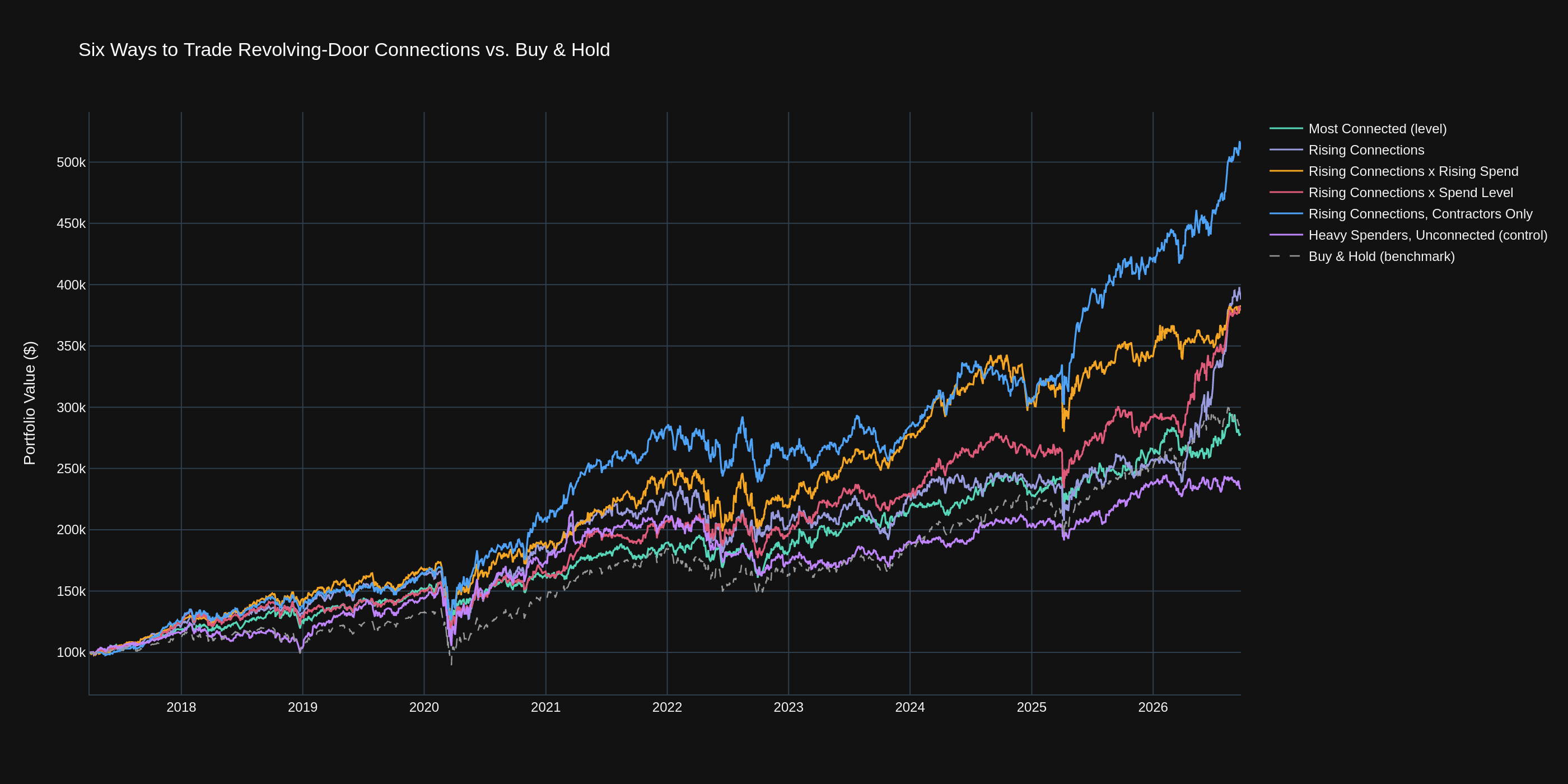
Editor's Note: every figure below comes from a real run on September 23, 2026 against live Quiver data, with prices through September 22. All six contestants are scored over the same window, March 31, 2017 to September 22, 2026, which is 38 quarterly rebalances. Numbers are reported as they came out, including the ones that argue against the thesis.
| Contestant | Return | Benchmark | Max DD | Sharpe | Win Rate | Holdings | Turnover |
|---|---|---|---|---|---|---|---|
| Most Connected (level) | +178.5% | +192.3% | 25.6% | 0.79 | 83% | 10 | 20% |
| Rising Connections | +287.9% | +192.3% | 32.3% | 0.88 | 63% | 10 | 67% |
| Rising Connections × Rising Spend | +281.8% | +192.3% | 25.8% | 0.94 | 65% | 10 | 76% |
| Rising Connections × Spend Level | +278.8% | +192.3% | 23.9% | 0.98 | 66% | 10 | 62% |
| Rising Connections, Contractors Only | +410.0% | +192.3% | 25.4% | 1.13 | 69% | 10 | 67% |
| Heavy Spenders, Unconnected (control) | +133.0% | +192.3% | 31.5% | 0.64 | 76% | 10 | 31% |
The control lost, and everything connected beat it
Start with the row that sets the bar. Heavy lobbying spenders with no revolving-door hires returned 133% and lost to the market by 59 points with the deepest drawdown in the field. Their book was Charter, Alphabet, American Electric Power, Meta, Anthem, AmerisourceBergen and Dominion: cable, utilities and healthcare distribution, plus two tech names that lobby heavily but had no connected lobbyists in most windows.
Every contestant that required connections beat that control, by 46 points for the static ranking and by 146 to 277 points for the change-based ones. Among companies that spend real money in Washington, having former government staff on the payroll separated the winners from the losers over a decade. That is the thesis, and it held.
Static connections are not enough
Most Connected beat the control but lost to the market, returning 179% against 192% with a lower drawdown. It held Comcast for all 38 quarters, Amgen for 37, General Dynamics for 32, Microsoft for 28 and T-Mobile for 27. Those are the companies with the largest permanent Washington presence, and the market has known that for decades. The portfolio kept pace through 2019 and then missed most of 2021 and 2024, the years the index was led by companies whose Washington footprint was still small.
A static connection count is a description of who is big and regulated. It is not a signal.
Change beats level, but read the fine print
Rising Connections returned 288% against 192%, a clear improvement on the static ranking. Almost all of that edge arrived in 2026. Through the end of 2025 it had returned about 157% against the benchmark's 150%, a dead heat over eight and three quarter years. Then its first-quarter 2026 portfolio held AMD, which returned 186% in a single quarter, along with Teradyne at 63%, and its second-quarter portfolio caught Marathon Petroleum, Phillips 66 and Workday. One year, and mostly one stock, is the difference between "matched the market" and "beat it by 96 points."
It also has the deepest drawdown of the connected contestants at 32% and the widest spread of holdings, 160 different companies over the decade. On its own, the change signal is noisy.
Pairing change with lobbying spend is where the edge gets steady
The two blends returned 282% and 279% with the two best drawdowns in the field, 26% and 24% against the market's roughly 35% in the COVID crash, and Sharpe ratios of 0.94 and 0.98. Unlike Rising Connections on its own, they do not depend on 2026. Through the end of 2025, Rising Connections × Rising Spend had returned about 241% against the benchmark's 150%, and it beat the market in five of nine full calendar years, including 2018 when it gained 16% while the market lost 7%.
Their holdings look different from the static portfolio too. Rising Connections × Rising Spend traded 155 companies and its most-held names, Abbott, Lockheed, Cigna, Amgen and Gilead, each appear in fewer than a quarter of the rebalances. It is finding companies at the moment their Washington effort steps up, not the ones that are always there.
Connections matter most where government is the customer
Rising Connections restricted to federal contractors is the result of this test. It returned 410% against 192%, with a Sharpe ratio of 1.13, a 25% maximum drawdown and a 69% win rate across 380 position-quarters. It beat the market in seven of ten calendar years, including both down years: it lost 8% in 2022 when the market lost 11%, and gained 11% in 2018 when the market lost 7%.
The holdings log is what makes it credible. It traded 124 different companies, and its largest single contributor, Micron, accounts for about 13 points of the 410. Amazon, GE, Qualcomm, Live Nation and JPMorgan follow closely. There is no AMD-sized outlier doing the work. Its recent portfolios read like a plausible list of companies where a new Washington hire could matter: Boeing, Northrop, Deere, Corning, Ameren, DTE, Axon, Broadcom.
Year by year
| Contestant | 2017 | 2018 | 2019 | 2020 | 2021 | 2022 | 2023 | 2024 | 2025 | 2026 |
|---|---|---|---|---|---|---|---|---|---|---|
| Most Connected (level) | +19% | +6% | +20% | +8% | +16% | -4% | +19% | +6% | +16% | +5% |
| Rising Connections | +20% | +10% | +24% | +14% | +23% | -12% | +13% | +3% | +9% | +51% |
| Rising Connections × Rising Spend | +24% | +16% | +17% | +14% | +29% | -10% | +27% | +10% | +12% | +12% |
| Rising Connections × Spend Level | +23% | +5% | +16% | +11% | +25% | -5% | +17% | +14% | +12% | +30% |
| Rising Connections, Contractors Only | +24% | +11% | +19% | +28% | +35% | -8% | +9% | +7% | +37% | +22% |
| Heavy Spenders, Unconnected (control) | +16% | -10% | +39% | +21% | +21% | -18% | +10% | +7% | +17% | -2% |
| Buy & Hold (benchmark) | +12% | -7% | +27% | +10% | +26% | -11% | +15% | +15% | +15% | +17% |
Read across the rows and the shape of each result is visible. The contractors-only portfolio beat the market in most years and in both bear years. The two blends were consistent rather than spectacular. Rising Connections on its own matched the market until 2026. Most Connected was rarely bad and rarely good. The control fell behind in 2018 and 2022 and never recovered the gap.
The window covers a full cycle: the 2018 fourth-quarter correction, the COVID crash and recovery, the 2022 rate-driven bear market, the narrow AI-led rally of 2023 and 2024, the April 2025 tariff selloff and its fast reversal, and the record run through 2026. A signal that only works in one regime shows up as one or two standout years. The contractors result and the two blends do not look like that.
Why this might work
The results narrow the theory rather than confirming it wholesale. What predicted returns was adding connections at companies whose business runs through Washington: heavy lobbyists, and above all federal contractors. A defense or infrastructure company hiring a former appropriations staffer is making an investment with a measurable payoff, a contract award, and the filing that discloses the hire is public months before the award. A consumer company hiring the same person is buying goodwill with no revenue line attached. The market may price the second kind of hire correctly and be slow on the first.
The decade of data also strengthens the case against static rankings. The most-connected companies in absolute terms are the largest regulated incumbents, and their Washington presence is a fact about their size, not news.
Risks & Caveats
- Six contestants is still a multiple-comparisons problem. With several entrants, the best one is partly the luckiest one, even over 38 rebalances. The contractors result deserves attention because it is consistent across years and spread across many trades, but it is one backtest on one universe. Re-test it on a different universe before believing it.
- Rising Connections' headline is one year. Its 96-point lead over the benchmark was a 7-point lead at the end of 2025. AMD's 186% quarter in early 2026 appears in four of the five connected portfolios.
- The direction of the change is not the whole story. In a wider run of this same pipeline we also tested the inverse of Rising Connections, companies shedding connected lobbyists, and it beat the market too. A changing roster in either direction identifies active, growing companies. The blends and the contractors filter survive that objection; Rising Connections on its own does not.
- The membership file treats renames as exits. Priceline becoming Booking appears as one company leaving the index and another joining. The benchmark carries the old symbol at its exit price and misses the new one's run. The effect is small at 1/500th weight, and it runs against the benchmark.
- Delisted holdings are carried at their last print. A stock acquired mid-quarter is held at its final price until the next rebalance sells it, which approximates the cash-out. A stock that went to zero would be frozen instead, a small upward bias for the strategies.
- The revolving-door feed begins in 2016. The first change trade is in early 2017, so nothing here is tested on the 2008 crisis or the years before 2016.
Other Ideas for you to Explore
- Re-test the contractors result on a different universe. Swap the S&P 500 membership file for the S&P 400 mid-caps, where a single connected hire is a larger share of a company's Washington effort. If the effect is real it should be at least as strong there.
- Drop the best trade and re-score. Remove each contestant's single best quarterly holding and report the return without it. Rising Connections should fall hard; the contractors-only portfolio should barely move.
- Run the inverse yourself. Rank by the most negative change in connections, restricted to companies that had a roster to lose. It is one line of code, and it is the fastest way to find out whether a signal is about direction or just about activity.
- Weight new hires by where they came from. The feed's
Branch,ChamberandFormerEmployerfields distinguish an appropriations committee staffer from an agency press officer. Match the former employer against the agencies a contractor sells to. - Shorten the lag for the contractors portfolio. Filings post within twenty days of quarter-end, so a monthly rebalance with a one-month lag would trade the same information two months sooner. Check whether the extra turnover is paid for.