TL;DR — What Worked and What Didn't
This tutorial pulls SEC Form 4 filings from the Quiver Insider Trading API,
filters them down to genuine open-market purchases (transaction code P, excluding
grants, option exercises, and tax withholding), and backtests five different ways of ranking
those purchases across the S&P 500 — monthly rebalance, 10 equal-weighted positions,
3-month lookback, one-month execution lag.
Results over 62 monthly rebalances (August 2021 – August 2026):
- Dollar value + 200-day uptrend filter: +78.5%, 15.5% max drawdown, 0.75 Sharpe — the only variant that beat the benchmark, and it did so with the shallowest drawdown of the six.
- Buy & hold, same universe: +57.3% — the bar every strategy had to clear.
- Raw insider dollar value: +57.6% — tied the market, but with a 22.6% drawdown instead of 15.5%.
- Executives only: +25.3%. Stake increase: +15.9%. Cluster buying: +7.1% — all three lost, badly.
Three findings worth the read: cluster buying (ranking by how many insiders bought) failed in large caps because it selects for companies with routine director purchase programs, not conviction. Filtering to officers only threw out the single best signal in the data — Berkshire Hathaway's 10%-owner buying of Occidental Petroleum. And two post-hoc attempts to cut the winner's high turnover both made it substantially worse, because the trend filter's sell rule was doing much of the work.
What you'll need: a Quiver Trader plan (Insider Trading is a Tier 2 dataset), a price data source, and Python with pandas and vectorbt. The complete script is linked below.
Company insiders have to disclose it within two business days whenever they buy or sell their own company's stock. Most of what gets filed isn't a signal at all — stock grants, option exercises, and tax-related share withholding all show up in the same feed as genuine purchases, and none of those reflect an insider actually spending their own money on the stock.
Every strategy in this tutorial starts from the same filtered feed — open-market purchases only — and plays by the same rules: rebalance monthly, hold up to 10 S&P 500 companies at equal weight, rank over a rolling 3-month window, act with a one-month lag. The only thing that changes between them is how each one decides which 10 companies deserve a spot.
That's deliberate. It turns this into a controlled experiment: five different hypotheses about what makes an insider purchase informative, each tested against the others and against a plain buy-and-hold benchmark, with everything else held constant. Think of it as a tournament — and before any results come in, each contestant states up front why it expects to win.
Getting Set Up with the Quiver API
To build this strategy you need a reliable source of insider transaction filings, not just a summary of the highlights.
Quiver's Insider Trading API gives you the full Form 4 filing feed — every transaction code, not just the ones a headline would mention — which is what makes it possible to filter down to genuine open-market purchases in the first place.
This section covers everything you need before writing strategy code: an account and key, how authentication works, and an important plan-tier detail this dataset requires that the other Quiver tutorials don't.
1. Create an account and grab your API key
Every Quiver endpoint requires authentication — there's no anonymous or free-tier data access.
Without a valid key, every call below returns a 401.
Head to the Quiver API pricing page to create an account and pick a plan.
Insider Trading is a Tier 2 dataset, which means it requires the Trader plan ($75/mo, or $62.50/mo billed annually) — the Hobbyist plan used in some other Quiver tutorials doesn't include it.
Use code 50YEAR at signup for 50% off your first year.
pip install requests pandas

# Store your key as an environment variable rather than hardcoding it
export QUIVER_API_KEY="your_key_here"
2. Authentication
Quiver's API authenticates via a bearer token in the Authorization header.
Before building anything, make one throwaway call to confirm the key works and that you're sending auth the way the API currently expects.
import os
import requests

API_KEY = os.environ["QUIVER_API_KEY"]
BASE_URL = "https://api.quiverquant.com"
HEADERS = {"Authorization": f"Bearer {API_KEY}"}

# Sanity-check call — note the date format below, it's unusual for this endpoint
resp = requests.get(f"{BASE_URL}/beta/live/insiders", headers=HEADERS, params={"date": "20240102", "page_size": 5})
print(resp.status_code)
print(resp.json()[:2])YYYY-MM-DD. This one doesn't — the Insider Trading endpoint expects YYYYMMDD with no dashes. Sending the usual format won't necessarily error, but it can silently return nothing, which is a confusing way to discover the difference. Confirm this with a real call before building a backfill loop around it.3. There's no historical or bulk endpoint — only live
This is a real, load-bearing difference from every other dataset used across these tutorials. Corporate Lobbying and Congress Trading both expose a per-ticker historical endpoint, so backfilling means looping over tickers. Insider Trading only exposes /beta/live/insiders, which takes a date parameter and returns that day's filings across every ticker at once.
That flips the backfill entirely: instead of looping over ~600 tickers, you loop over every trading day in the backtest window — around 2,000 calls for a multi-year backtest, meaningfully more than the ticker-based approach elsewhere. Budget more time for this one.
4. Confirm how far back the data actually goes
The endpoint's own description calls it "recent insider transactions" — worth taking seriously before committing to years of backfill. Test a handful of old dates first.
# Spot-check historical depth before committing to a multi-year backfill
for test_date in ["20180102", "20200102", "20220103"]:
    resp = requests.get(f"{BASE_URL}/beta/live/insiders", headers=HEADERS, params={"date": test_date, "page_size": 5})
    rows = resp.json()
print(test_date, "->", len(rows), "filings returned")BACKTEST_START below to whatever the data actually supports rather than backfilling years of empty responses.Pulling the Data
Same point-in-time S&P 500 universe as any broad-universe strategy: use today's constituent list applied retroactively and you get survivorship bias, so pull real historical membership instead.
import pandas as pd
import datetime

SP500_HIST_URL = (
    "https://raw.githubusercontent.com/fja05680/sp500/master/"
    "S%26P%20500%20Historical%20Components%20%26%20Changes%20(Updated).csv"
)
sp500_hist = pd.read_csv(SP500_HIST_URL, parse_dates=["date"]).sort_values("date")

def sp500_members_asof(date, hist=sp500_hist):
    """S&P 500 tickers as of `date`, using the most recent snapshot on or
    before it — only ever reflects membership that was public knowledge
    on that date, which is what avoids look-ahead/survivorship bias."""
    row = hist[hist["date"] <= pd.Timestamp(date)].iloc[-1]
    return set(row["tickers"].split(","))

BACKTEST_START = "2018-01-01"  # shorten this if the coverage check above found gaps
BACKTEST_END = (datetime.date.today() - datetime.timedelta(days=1)).isoformat()
Now the backfill itself — looping over dates, not tickers.
import time

def get_with_retry(url, params=None, max_retries=5):
    """Returns None once retries are exhausted, not a raised exception — a
    single persistently-failing date shouldn't crash a multi-hour backfill.
    Retries on 429 (rate limit) AND any 5xx."""
    for attempt in range(max_retries):
        resp = requests.get(url, headers=HEADERS, params=params)
        if resp.status_code == 200:
            return resp.json()
        if resp.status_code == 429 or resp.status_code >= 500:
            wait = 2 ** attempt
            print(f"  {resp.status_code} error on attempt {attempt + 1}/{max_retries}, retrying in {wait}s...")
            time.sleep(wait)
            continue
        print(f"Error {resp.status_code} on {url}: {resp.text[:500]}")
        resp.raise_for_status()
    print(f"  Giving up on {url} after {max_retries} retries")
    return None

def paginate(url, params=None, page_size=250):
    params = dict(params or {})
    params["page_size"] = page_size
    page, all_rows = 1, []
    while True:
        params["page"] = page
        rows = get_with_retry(url, params)
        if rows is None or not rows:
            break
        all_rows.extend(rows)
        if len(rows) < page_size:
            break
        page += 1
    return all_rows

def backfill_insiders(start, end, pause=0.25, checkpoint_every=200, checkpoint_path="insiders_backfill_checkpoint.csv"):
    """Loops over business days, not tickers — this dataset only exposes a
    live/current endpoint with a date parameter, no per-ticker history."""
    trading_days = pd.bdate_range(start, end)
    all_rows, failed_dates = [], []
    for i, day in enumerate(trading_days):
        date_str = day.strftime("%Y%m%d")  # YYYYMMDD, not YYYY-MM-DD, for this endpoint
        url = f"{BASE_URL}/beta/live/insiders"
        rows = paginate(url, {"date": date_str})
        if not rows:
            failed_dates.append(date_str)
        all_rows.extend(rows)
        time.sleep(pause)
        if i % 50 == 0:
            print(f"  {i}/{len(trading_days)} days pulled ({len(all_rows)} filings so far)")
        if i > 0 and i % checkpoint_every == 0:
            pd.DataFrame(all_rows).to_csv(checkpoint_path, index=False)
            print(f"  Checkpoint saved to {checkpoint_path} ({len(all_rows)} rows)")
    if failed_dates:
        print(f"\nNo data returned for {len(failed_dates)} dates (holidays, gaps, or failures)")
    return all_rows

raw_rows = backfill_insiders(BACKTEST_START, BACKTEST_END)
insiders_df = pd.DataFrame(raw_rows)
print(insiders_df.columns.tolist()) # confirm actual field names before referencing themBuilding the Signal
Download and clean price data first.
import vectorbt as vbt

POLYGON_API_KEY = os.environ["POLYGON_API_KEY"]
POLYGON_BASE_URL = "https://api.polygon.io"

def get_polygon_with_retry(url, params=None, max_retries=5):
    for attempt in range(max_retries):
        resp = requests.get(url, params=params)
        if resp.status_code == 200:
            return resp.json()
        if resp.status_code == 429 or resp.status_code >= 500:
            wait = 2 ** attempt
            print(f"  {resp.status_code} error on attempt {attempt + 1}/{max_retries}, retrying in {wait}s...")
            time.sleep(wait)
            continue
        print(f"Error {resp.status_code} on {url}: {resp.text[:500]}")
        resp.raise_for_status()
    print(f"  Giving up on {url} after {max_retries} retries")
    return None

def download_price_polygon(tickers, start, end, pause=0.25):
    series = {}
    for i, ticker in enumerate(tickers):
        url = f"{POLYGON_BASE_URL}/v2/aggs/ticker/{ticker}/range/1/day/{start}/{end}"
        params = {"adjusted": "true", "sort": "asc", "limit": 50000, "apiKey": POLYGON_API_KEY}
        data = get_polygon_with_retry(url, params)
        results = (data or {}).get("results") or []
        if results:
            df = pd.DataFrame(results)
            df["date"] = pd.to_datetime(df["t"], unit="ms")
            series[ticker] = df.set_index("date")["c"]
        time.sleep(pause)
    return pd.DataFrame(series)
Clean ticker strings before using them anywhere downstream, and filter to genuine open-market purchases — not the whole Form 4 feed.
import re

def clean_ticker(raw_ticker):
    """Quiver's insider feed occasionally has exchange-prefixed or
    parenthesized ticker strings (e.g. "(NYSE:FBC)") instead of a plain
    symbol. Strip that down to just the ticker, or return None if it still
    doesn't look like a real one."""
    if not isinstance(raw_ticker, str):
        return None
    t = raw_ticker.strip().strip("()")
    if ":" in t:
        t = t.split(":")[-1]
    t = t.strip().upper()
    return t if re.fullmatch(r"[A-Z]{1,6}(\.[A-Z])?", t) else None

insiders_df["Ticker"] = insiders_df["Ticker"].apply(clean_ticker)
insiders_df = insiders_df.dropna(subset=["Ticker"])

# TransactionCode "P" is an open-market or private purchase — the SEC Form 4
# code for an insider actually buying shares with their own money. Grants
# ("A"), option exercises ("M"), tax withholding ("F"), and gifts ("G") all
# also show up as "acquisitions" in this feed but aren't a discretionary bet
# on the stock, so they're excluded here.
insiders_df["fileDate"] = pd.to_datetime(insiders_df["fileDate"])
purchases = insiders_df[insiders_df["TransactionCode"] == "P"].copy()
print(f"Genuine open-market purchases: {len(purchases)} of {len(insiders_df)} total filings")"(NYSE:FBC)" instead of a plain ticker, and passing that straight into a price API call fails outright (a 404, "ticker prefix does not exist") rather than just being wrong. Confirmed directly.Scope the price pull to the intersection of purchase tickers and the point-in-time S&P 500 window — the insider feed covers the whole market, not just the S&P 500.
# The insider feed covers the whole market, not just the S&P 500 — pulling
# price data for every ticker that ever had a purchase means pulling for
# thousands of names instead of a few hundred, almost all of which this
# strategy will never trade. Intersect with the S&P 500 window first.
window = sp500_hist[(sp500_hist["date"] >= BACKTEST_START) & (sp500_hist["date"] <= BACKTEST_END)]
sp500_universe = set().union(*window["tickers"].str.split(","))

universe = sorted(set(purchases["Ticker"].dropna().unique()) & sp500_universe)
price = download_price_polygon(universe, BACKTEST_START, BACKTEST_END)
price = price.dropna(axis=1, how="all").astype(float)
print(f"Price data returned for {price.shape[1]} of {len(universe)} tickers")
With the data cleaned and scoped, one more shared preparation step before the contestants diverge: derive the columns the different ranking rules will need, compute a 200-day moving average for the trend-filter variant, and set two parameters that matter more than they look.
MAX_POSITIONS = 10
RANKING_LOOKBACK_MONTHS = 3
INIT_CASH = 100_000

# "auto" = start the portfolio (and the benchmark) on the first day ANY
# variant actually trades. See the callout below for why this matters.
PORTFOLIO_START = "auto"

monthly_index = pd.date_range(BACKTEST_START, BACKTEST_END, freq="ME")

# The API returns real booleans, but a CSV round-trip through the checkpoint
# file turns them into strings — coerce robustly either way
for col in ["isOfficer", "isDirector", "isTenPercentOwner"]:
    if col in purchases.columns:
        purchases[col] = purchases[col].astype(str).str.lower().eq("true")

purchases["Value"] = purchases["Shares"] * purchases["PricePerShare"]

# How much did this purchase grow the insider's EXISTING position? Capped at
# 1.0 (a 100% increase) so an insider going from ~0 shares to a real position
# doesn't produce an absurd ratio that swamps everything else.
prior_holdings = (purchases["SharesOwnedFollowing"] - purchases["Shares"]).clip(lower=1)
purchases["StakeIncrease"] = (purchases["Shares"] / prior_holdings).clip(upper=1.0)

# 200-day moving average from past prices only — no look-ahead. Computed on
# the full price history so it's already warmed up when trading begins.
ma200 = price.rolling(200, min_periods=200).mean()

membership_by_month = {m_end: sp500_members_asof(m_end) for m_end in monthly_index}

# Annualize ratio metrics (Sharpe, Sortino, Calmar) on trading days
vbt.settings.returns["year_freq"] = "252 days"Five Ways to Read the Same Data
Each contestant is a single function that takes the purchases filed in the trailing 3-month window and returns one score per company. Higher score, better rank. Everything downstream — the top-10 cut, the equal weights, the rebalancing — is shared.
Before looking at any results, each contestant states its hypothesis. That matters more than it sounds: writing down what you expect to win before you run the test is the difference between learning something and just picking whichever line ended up highest on the chart. It also makes the results section below honest — each hypothesis gets a verdict, including the ones that lost.
Contestant 1 — Dollar Value (the baseline)
"The more money insiders put down, the more they know."
The simplest reading: rank companies by the total dollars insiders spent buying. It's the natural first guess, and it's the bar the other four have to clear.
def rank_by_dollar_value(window_purchases):
    return window_purchases.groupby("Ticker")["Value"].sum()
Contestant 2 — Cluster Buying
"Several insiders agreeing beats one insider going big."
One executive making a large purchase might be rebalancing their personal finances. Three or four different insiders all buying in the same quarter is harder to explain away — each of them sees the company from the inside, and they independently reached the same conclusion. Lakonishok and Lee's 2001 study found this kind of consensus among insiders carries more predictive information than any single purchase. This variant ranks by the number of distinct people who bought (using the Name field), with dollar value only as a tie-breaker.
def rank_by_cluster_buying(window_purchases):
    distinct_buyers = window_purchases.groupby("Ticker")["Name"].nunique()
    dollar_value = window_purchases.groupby("Ticker")["Value"].sum()
    return distinct_buyers + (dollar_value / dollar_value.max()).fillna(0) * 0.5
Contestant 3 — Executives Only
"The CEO's buy means more than a director's."
Not all insiders are equally inside. Officers — the CEO, CFO, and other executives — run the business day to day and see the numbers before anyone else. Outside directors show up for board meetings; 10% owners may be funds with their own reasons to trade. Seyhun's research found top executives' trades are meaningfully more informative than those of directors or large shareholders. This variant uses the same dollar-value ranking as the baseline but counts only purchases where isOfficer is true.
def rank_by_executives_only(window_purchases):
    officers = window_purchases[window_purchases["isOfficer"]]
    return officers.groupby("Ticker")["Value"].sum()
Contestant 4 — Stake Increase (conviction)
"How much they spent matters less than how much it changed their bet."
A billionaire founder adding $2 million to a $2 billion position is a rounding error. A division president spending $200,000 when she already owns $150,000 worth just more than doubled her exposure to her own company's future. Dollar value can't tell those two apart; this variant can. It ranks by the total relative increase in insiders' existing stakes, which also strips out the size bias — the baseline structurally favors mega-caps and wealthy insiders, and this doesn't.
def rank_by_stake_increase(window_purchases):
    return window_purchases.groupby("Ticker")["StakeIncrease"].sum()
Contestant 5 — Dollar Value + Uptrend Filter
"Insider buying works — unless they're catching a falling knife."
An earlier version of this strategy found its biggest losers were companies in long, structural declines: an insider buying because they believed the stock was cheap, and being wrong because the business itself was deteriorating. This variant keeps the baseline dollar-value ranking but only allows companies trading above their own 200-day moving average — insider buying plus a stock that's already turned up, rather than insider buying into a slide. It's the classic "smart money agreeing with the tape" combination.
# uptrend_mode: None     -> no trend filter
#               "always" -> must be above its 200-day MA to be held at all
#               "entry"  -> must be above its 200-day MA to be ADDED (used in Round 2)
VARIANTS = {
    "Dollar Value (baseline)":       {"rank": rank_by_dollar_value,    "uptrend_mode": None},
    "Cluster Buying":                {"rank": rank_by_cluster_buying,  "uptrend_mode": None},
    "Executives Only":               {"rank": rank_by_executives_only, "uptrend_mode": None},
    "Stake Increase (conviction)":   {"rank": rank_by_stake_increase,  "uptrend_mode": None},
    "Dollar Value + Uptrend Filter": {"rank": rank_by_dollar_value,    "uptrend_mode": "always"},
}
The Shared Rules
Three functions do the same work for every contestant. The first turns a ranking function into a monthly "which 10 companies" grid; the second finds the first day a variant actually trades; the third turns the grid into a backtest that begins on the shared start date.
def build_qualifies(rank_fn, uptrend_mode=None, sticky_rank=None):
    qualifies = pd.DataFrame(False, index=monthly_index, columns=price.columns)
    prev_held = set()
    for m_end in monthly_index:
        m_start = m_end - pd.DateOffset(months=RANKING_LOOKBACK_MONTHS) + pd.Timedelta(days=1)
        window_purchases = purchases[
            (purchases["fileDate"] >= m_start) & (purchases["fileDate"] <= m_end)
        ]
        scores = rank_fn(window_purchases).sort_values(ascending=False)
        members = membership_by_month[m_end]
        candidates = [t for t in scores.index if t in price.columns and t in members]

        in_uptrend = None
        if uptrend_mode is not None:
            pos = price.index.searchsorted(m_end, side="right") - 1
            if pos >= 0:
                asof = price.index[pos]
                in_uptrend = price.loc[asof] > ma200.loc[asof]

        if uptrend_mode == "always":
            if in_uptrend is not None:
                candidates = [t for t in candidates if bool(in_uptrend.get(t, False))]
            selected = candidates[:MAX_POSITIONS]
        elif uptrend_mode == "entry":
            # Existing holdings are kept if still ranked; only NEW names need the uptrend
            keep_pool = candidates[:sticky_rank] if sticky_rank else candidates[:MAX_POSITIONS]
            kept = [t for t in keep_pool if t in prev_held]
            new = [t for t in candidates
                   if t not in kept and (in_uptrend is None or bool(in_uptrend.get(t, False)))]
            selected = (kept + new)[:MAX_POSITIONS]
        else:
            selected = candidates[:MAX_POSITIONS]

        qualifies.loc[m_end, selected] = True
        prev_held = set(selected)
    return qualifies


def first_trade_day(qualifies):
    has_holdings = qualifies.sum(axis=1) > 0
    if not has_holdings.any():
        return None
    first_signal_month = has_holdings[has_holdings].index[0]
    lag_month_pos = monthly_index.get_loc(first_signal_month) + 1  # the one-month lag
    if lag_month_pos >= len(monthly_index):
        return None
    pos = price.index.searchsorted(monthly_index[lag_month_pos])
return price.index[pos] if pos < len(price.index) else NonefileDate — when the purchase became public — not the transaction date, since SEC rules give insiders up to two business days to file. And the 3-month lookback matters: at a 1-month lookback, an earlier version of this strategy's top-10 list turned over roughly 62% every month, because a single large purchase can win one month's ranking and never repeat. Three months roughly halves that, giving sustained buying a chance to keep a company in the portfolio long enough to compound.def run_backtest(qualifies, start):
target_weights = pd.DataFrame(0.0, index=monthly_index, columns=qualifies.columns)
for m_end in monthly_index:
selected = qualifies.columns[qualifies.loc[m_end]]
if len(selected) > 0:
target_weights.loc[m_end, selected] = 1.0 / len(selected)
target_weights = target_weights.shift(1).fillna(0.0) # one month of execution lag
size = pd.DataFrame(float("nan"), index=price.index, columns=price.columns)
for m_end, row in target_weights.iterrows():
pos = price.index.searchsorted(m_end)
if pos < len(price.index):
size.loc[price.index[pos]] = row.values
# Slice BOTH price and size to the shared start, so the benchmark is
# measured over the same window as the strategy
price_bt = price.loc[start:]
size_bt = size.loc[start:]
portfolio = vbt.Portfolio.from_orders(
price_bt, size=size_bt, size_type="targetpercent",
init_cash=INIT_CASH, fees=0.0, slippage=0.0002,
group_by=True, cash_sharing=True, freq="1D",
)
# Monthly holdings snapshot: what was held, at what weight, how it did
rebalance_days = size_bt.dropna(how="all").index.tolist()
rows = []
for i, day in enumerate(rebalance_days):
held = size_bt.loc[day][size_bt.loc[day] > 0]
next_day = rebalance_days[i + 1] if i + 1 < len(rebalance_days) else price_bt.index[-1]
for ticker, w in held.items():
rows.append({
"Rebalance Date": day.date(), "Ticker": ticker, "Weight": round(w, 4),
"Return": round(price_bt.loc[next_day, ticker] / price_bt.loc[day, ticker] - 1, 4),
})
holdings_history = pd.DataFrame(rows)
# Month-over-month persistence of the selection, over months actually traded
q_live = qualifies.loc[qualifies.index >= pd.Timestamp(start) - pd.DateOffset(months=1)]
months = q_live.index.tolist()
overlaps = []
for i in range(1, len(months)):
prev = set(q_live.columns[q_live.loc[months[i - 1]]])
curr = set(q_live.columns[q_live.loc[months[i]]])
if prev:
overlaps.append(len(prev & curr) / len(prev))
avg_turnover = 1 - (sum(overlaps) / len(overlaps)) if overlaps else float("nan")
avg_holdings = q_live.sum(axis=1)[q_live.sum(axis=1) > 0].mean()
return portfolio, holdings_history, avg_turnover, avg_holdingssize_type="targetpercent" is what makes every contestant compound for real: each monthly rebalance targets a percentage of the current portfolio value, so gains flow into the size of next month's positions automatically. This is NOT the same as size_type="percent", which sizes off remaining cash processed ticker by ticker and quietly produces a lopsided, non-equal allocation — confirmed by testing it directly. fees=0.0, slippage=0.0002 reflect how this would actually be traded: $0 commission is standard at every major US retail broker, and 2 basis points is a modest, slightly conservative stand-in for spread and impact on a $10-25k trade in a liquid S&P 500 name.freq="1D" argument isn't cosmetic. Real price data has no fixed frequency — weekends and holidays are missing, so pandas can't infer one — and without an explicit frequency, vectorbt silently leaves Sharpe, Sortino, and Calmar out of stats(). Confirmed the hard way: the first live scorecard for this tournament came back with an empty Sharpe column. Together with the year_freq = "252 days" setting above, this annualizes those ratios on trading days.Running the Tournament
Find the shared start, then run every contestant through the same pipeline and put the numbers side by side.
def run_round(variants, start, label):
    results = {}
    for name, cfg in variants.items():
        qualifies = build_qualifies(cfg["rank"], cfg.get("uptrend_mode"), cfg.get("sticky_rank"))
        portfolio, holdings_history, avg_turnover, avg_holdings = run_backtest(qualifies, start)
        slug = name.lower().replace(" ", "_").replace("(", "").replace(")", "").replace("+", "plus").replace(",", "")
        holdings_history.to_csv(f"holdings_history_{slug}.csv", index=False)
        stats = portfolio.stats()
        results[name] = {
            "portfolio": portfolio,
            "Total Return [%]": stats["Total Return [%]"],
            "Benchmark Return [%]": stats["Benchmark Return [%]"],
            "Max Drawdown [%]": stats["Max Drawdown [%]"],
            "Sharpe Ratio": stats.get("Sharpe Ratio", float("nan")),
            "Win Rate [%]": stats["Win Rate [%]"],
            "Avg Holdings": avg_holdings,
            "Monthly Turnover [%]": avg_turnover * 100,
        }
    scorecard = pd.DataFrame({k: {kk: vv for kk, vv in v.items() if kk != "portfolio"} for k, v in results.items()}).T
    print(scorecard.round(2).to_string())
    scorecard.round(4).to_csv(f"variant_scorecard_{label.lower().replace(' ', '_')}.csv")
    return results, scorecard

# Shared start: the first day any contestant actually trades
if PORTFOLIO_START == "auto":
    starts = []
    for cfg in VARIANTS.values():
        q = build_qualifies(cfg["rank"], cfg.get("uptrend_mode"), cfg.get("sticky_rank"))
        d = first_trade_day(q)
        if d is not None:
            starts.append(d)
    portfolio_start = min(starts)
else:
    portfolio_start = pd.Timestamp(PORTFOLIO_START)
print(f"Portfolio start (shared by all variants and the benchmark): {portfolio_start.date()}")

round1_results, round1_scorecard = run_round(VARIANTS, portfolio_start, "Round 1")
Then one chart with every contestant on it, plus buy-and-hold — now measured over the same window — as the bar they all need to clear.
import plotly.graph_objects as go

def plot_round(results, title, image_id):
    palette = ["#57D7BA", "#999cde", "#f5a623", "#e05a7a", "#4fa3f7", "#c084fc"]
    fig = go.Figure()
    for (name, res), color in zip(results.items(), palette):
        value = res["portfolio"].value()
        fig.add_trace(go.Scatter(x=value.index, y=value.values, name=name, line=dict(color=color, width=1.6)))
    benchmark = next(iter(results.values()))["portfolio"].benchmark_value()
    fig.add_trace(go.Scatter(x=benchmark.index, y=benchmark.values, name="Buy & Hold (benchmark)",
                             line=dict(color="rgb(151,153,154)", width=1.2, dash="dash")))
    fig.update_layout(
        template="plotly_dark", paper_bgcolor="#121212", plot_bgcolor="#121212",
        font=dict(family="Figtree, sans-serif", color="rgb(241,243,244)"),
        xaxis=dict(gridcolor="#2F3F4D", linecolor="#2F3F4D"),
        yaxis=dict(gridcolor="#2F3F4D", linecolor="#2F3F4D", title="Portfolio Value ($)"),
        title=dict(text=title, font=dict(color="rgb(251,253,254)")),
        legend=dict(bgcolor="rgba(0,0,0,0)"),
    )
    fig.write_html(f"{image_id}.html")   # interactive version
    fig.write_image(f"{image_id}.png", width=1400, height=700, scale=2)  # needs: pip install kaleido
    fig.show()

plot_round(round1_results, "Five Ways to Trade Insider Buying", "round1-equity-curves")
Round 1 Results: The Verdicts
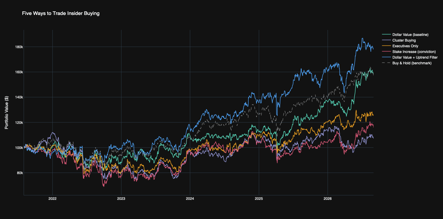
Round 1 was run against live Quiver and Polygon data. Trading began August 2, 2021 — the first month the insider feed had enough filings to fill a 3-month ranking window — and ran through August 2026: just over five years and 62 monthly rebalances. Every contestant and the buy-and-hold benchmark start on the same day at $100,000, so this is a fair fight.
| Contestant | Total Return | Max Drawdown | Sharpe | Win Rate | Turnover / mo | Verdict |
|---|---|---|---|---|---|---|
| Dollar Value + Uptrend Filter | +78.5% | 15.5% | 0.75 | 58.6% | 53.3% | Won — beat the benchmark by 21 points, best drawdown, best Sharpe |
| Buy & Hold (same universe) | +57.3% | — | — | — | — | The bar to clear |
| Dollar Value (baseline) | +57.6% | 22.6% | 0.59 | 63.3% | 35.2% | Tied the benchmark — with a worse ride |
| Executives Only | +25.3% | 23.1% | 0.34 | 60.5% | 36.5% | Lost to baseline and benchmark |
| Stake Increase (conviction) | +15.9% | 32.5% | 0.25 | 61.4% | 39.7% | Lost |
| Cluster Buying | +7.1% | 34.0% | 0.17 | 61.5% | 33.9% | Lost — badly |
Live results, August 2021 — August 2026, all contestants and the benchmark aligned to the same start date. Fees $0, slippage 2bps.
What the Scorecard Says About Each Hypothesis
The uptrend filter won, and the win is the real kind. Its hypothesis — that insider buying works except when the insider is catching a falling knife — produced the best return (+78.5% vs. +57.3% for buy-and-hold), the shallowest drawdown (15.5%, against 22–34% for everyone else), and the best Sharpe (0.75). It's the only contestant that clearly beat buy-and-hold. The holdings data shows how: its worst positions (Ford, Match, Norwegian Cruise Line, DXC) cost it a fraction of what the other four lost on PayPal, Nike, Walgreens, Warner Bros. Discovery, and VF Corp — all names in long structural declines that the trend filter kept it out of. That's the hypothesis working exactly as stated.
The baseline tied the benchmark almost to the decimal — +57.6% against +57.3% — but got there with a 22.6% drawdown versus the uptrend filter's 15.5%. Same destination, rougher road. Raw insider buying, on its own, roughly matched the market over this period without beating it. That is a useful and unglamorous finding.
Cluster Buying lost badly, and the holdings explain why. It held Simon Property Group in 61 of 62 months and Con Edison in 38. Those aren't companies with waves of conviction buying — they're companies where many directors make small, regular open-market purchases, most plausibly through standing director stock-purchase programs. A count of distinct buyers can't tell a coordinated bet from a routine payroll deduction. This is Cohen, Malloy, and Pomorski's "routine insider" problem showing up in the data, and it's a real caveat on the Lakonishok–Lee finding for this universe: in large-cap stocks, the companies with the most insiders buying may just be the companies with the most scheduled buying.
Executives Only lost to the baseline — the opposite of what Seyhun's research would predict. One likely reason is visible in what it excluded: the baseline's single most persistent holding was Occidental Petroleum (30 of 62 months), which appears in the feed as a 10%-owner purchaser — most plausibly Berkshire Hathaway's well-documented open-market buying of OXY over 2022–2024. Executives Only threw that out by design, and OXY was one of the baseline's better positions. Sometimes the biggest, most informed buyer is neither the CEO nor a director. Executives Only also dropped to as few as 2 holdings in some months, a concentration problem none of the other contestants had.
Stake Increase lost too. Normalizing away purchase size sounds right in principle, but in practice it promotes insiders with tiny prior holdings — a newly appointed director's first purchase registers as a 100% stake increase regardless of how small it is. Its worst positions were the same value traps that hurt the baseline (PayPal, WBD, VF Corp, Walgreens), plus Caesars, and it had the second-worst drawdown of the five.
One name did a lot of the winning for three contestants. Micron was the single largest contributor to the baseline, Stake Increase, and the uptrend filter alike — the AI-driven memory-chip rally of 2024–2026 found its way into the portfolio through insider purchases well before the biggest moves. Worth knowing: a chunk of each of those three contestants' returns traces back to one very good call.
What the Chart Shows
- August 2021 — late 2022: every contestant and the benchmark fell together into the 2022 bear market — the Fed's fastest rate-hiking cycle in four decades — bottoming in the $70–85k range. The uptrend filter's drawdown was visibly shallower; it simply held fewer of the names that fell hardest.
- 2023: a choppy, sideways recovery for all five, still tightly bunched, with the benchmark in the middle of the pack.
- 2024 — early 2025: the field separated. The uptrend filter pulled clear of the benchmark as the AI-led rally lifted names like Micron and Palo Alto Networks; the baseline tracked the benchmark closely; Cluster Buying and Stake Increase, anchored in slower-moving or declining names, fell behind and stayed there.
- Spring 2025: a sharp, brief drop hit every line at once — the tariff-driven correction — with the uptrend filter recovering fastest.
- Late 2025 — August 2026: the uptrend filter finished near $178k, the baseline and benchmark together near $160k, Executives Only around $125k, and Cluster Buying and Stake Increase in the $105–115k range.
Round 2: Trying to Refine the Winner (post-hoc)
The uptrend filter won Round 1 with one visible weakness: the highest turnover of any contestant, 53% a month. That's the always-on filter at work — a company that dips below its 200-day average gets sold even if insiders still rank it highly, then gets bought back when it recovers. Since churn had hurt earlier versions of this strategy, it looked like an obvious thing to fix.
Refinement A — Uptrend at Entry Only
"Require the uptrend to get in; don't sell on a routine dip."
A company must be above its 200-day average to be added, but once held, it stays as long as insiders still rank it in the top 10 — it isn't re-tested every month. The idea: keep the filter's protection against buying into declines, without forcing a sale every time a good position wobbles through its average.
Refinement B — Uptrend at Entry + Sticky Top-20
"Also stop churning names that slip one spot past the cutoff."
Same as A, plus an existing holding is retained if it's anywhere in the insider top 20, not just the top 10. A company ranked 9th one month and 11th the next shouldn't be sold and rebought over a marginal ranking change.
ROUND2_VARIANTS = {
    "Dollar Value + Uptrend Filter":    {"rank": rank_by_dollar_value, "uptrend_mode": "always"},
    "Uptrend at Entry Only":            {"rank": rank_by_dollar_value, "uptrend_mode": "entry"},
    "Uptrend at Entry + Sticky Top-20": {"rank": rank_by_dollar_value, "uptrend_mode": "entry", "sticky_rank": 20},
}
round2_results, round2_scorecard = run_round(ROUND2_VARIANTS, portfolio_start, "Round 2")
plot_round(round2_results, "Round 2: Refining the Winner (post-hoc)", "round2-equity-curves")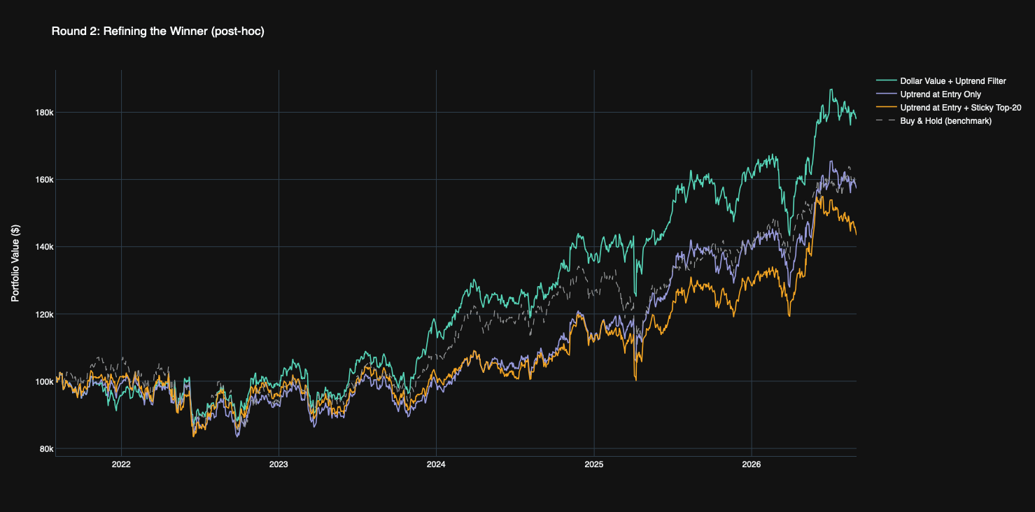
| Variant | Total Return | Max Drawdown | Sharpe | Turnover / mo | Verdict |
|---|---|---|---|---|---|
| Dollar Value + Uptrend Filter (Round 1 winner) | +78.5% | 15.5% | 0.75 | 53.3% | Still the winner |
| Uptrend at Entry Only | +57.3% | 18.7% | 0.62 | 48.1% | Worse on every measure but turnover |
| Uptrend at Entry + Sticky Top-20 | +43.4% | 19.1% | 0.50 | 44.0% | Worse still |
Live results, same window and start date as Round 1.
Round 2 Verdict: The "Churn" Was Doing the Work
Both refinements failed, and they failed in a way that teaches something Round 1 couldn't. Each one cut turnover a little — from 53% to 48% to 44% a month — and gave back a great deal in exchange: return fell from +78.5% to +57.3% to +43.4%, drawdown got worse, Sharpe fell from 0.75 to 0.50. Refinement A ended up almost exactly where the plain baseline did, which means letting positions ride through a trend break threw away essentially the entire benefit of having a trend filter at all.
The holdings explain the mechanism, and it's two things, not one.
First, the exit rule was protective, not noise. When the always-on filter sold a company that fell below its 200-day average, it was often getting out ahead of a real deterioration. The refinements kept holding those names as long as insiders still ranked them — and insiders kept ranking them, because insiders were still buying the dip. That's how Refinement A stayed in Enphase through the solar collapse, and Refinement B stayed in Albemarle through the lithium crash and in Archer-Daniels-Midland through its accounting scandal. In each case the insider signal said "hold" and the price trend said "leave," and the trend was right. The very trades that looked like churn were the filter cutting losers.
Second, a slot kept is a slot not given to someone better. Retaining a fading position means one fewer opening for a fresh, high-ranked company that's also in an uptrend. Royal Caribbean and NXP Semiconductors were two of the always-on filter's better positions; both refinements did meaningfully worse on them, not because they held them badly but because legacy positions were occupying the slots when those names would have entered. Stickiness has an opportunity cost that a turnover number doesn't show.
There's a broader lesson here about how to read a scorecard. Turnover looked like the winner's weakness because high turnover really had hurt earlier versions of this strategy. But turnover isn't bad in itself — uninformed turnover is bad. Rebalancing a portfolio because a noisy ranking reshuffled is costly churn; selling a position because its trend broke is a decision. The number looks the same in both cases. What separated them was only visible in the holdings.
One more honest note: on synthetic test data, the sticky refinement cut turnover by roughly 40%. On real data it cut it by 17%. Real insider rankings are noisier than a simulation, and a refinement tuned on a simulation should be expected to deliver less in practice than it promised.
How to Read the Scorecard
- Total Return vs. Benchmark — did it beat just buying and holding the same universe over the same window? Here that bar was +57.3%. A strategy that returned 40% lost, no matter how good 40% sounds on its own.
- Max Drawdown — the worst peak-to-trough drop along the way. This is the number that decides whether you'd actually have held on through the rough patch or bailed at the bottom. Cluster Buying's 34% drawdown means watching $100,000 become $66,000 and doing nothing.
- Sharpe Ratio — return per unit of volatility, or roughly, reward per unit of stomach-churn. The uptrend filter's 0.75 against the baseline's 0.59 says it earned its extra return without a rougher ride — it had a smoother one.
- Win Rate — what fraction of individual trades made money. Easy to over-read: the uptrend filter had the lowest win rate in Round 1 (58.6%) and still won, because its winners were bigger than its losers. Cluster Buying had a higher win rate and lost badly.
- Monthly Turnover — what fraction of the portfolio gets replaced each rebalance. Lower usually means positions stay long enough to compound — but Round 2 is a warning against treating it as a score to minimize. Some turnover is the strategy making good decisions.
Why This Might Work
Insiders have information about their own company that the market doesn't yet have, and buying shares on the open market is a costly, discretionary signal — unlike a grant or an option exercise, it means putting personal money at risk. Academic research on insider trading (Seyhun's work is the classic reference) has found open-market purchases carry more predictive information than sales, since insiders sell for all kinds of ordinary reasons — diversification, taxes, a house purchase — but usually only buy when they believe the stock is undervalued.
Round 1 sharpens that picture: the raw signal roughly matched the market but didn't beat it. It's real but blunt — it doesn't know the difference between an insider buying a temporary dip and one buying into a permanent decline. The single most effective thing tested here was giving it that distinction with a simple trend filter: the market's own verdict on the stock, layered on top of the insider's. Round 2 then showed the filter's value lives as much in when it sells as in what it buys.
Risks & Caveats
- Test five things and one will look good by luck. With five contestants, the best-performing one is partly the winner of a coin-flipping contest. The uptrend filter's win is more convincing than most — it won on return, drawdown, and Sharpe at once, the holdings show a clear mechanism, and two attempts to improve it both made it worse — but it's still one period and one universe. Treat it as a hypothesis worth re-testing, not a finished strategy.
- The benchmark comparison depends entirely on the start date. Measured from 2018, buy-and-hold crushed every contestant (186%). Measured fairly, from the first trade in August 2021, it returned 57.3% — and the baseline tied it while the uptrend filter beat it. "Beat the benchmark" is only meaningful when both start on the same day.
- Micron did a lot of the work. Three of the five contestants share the same top contributor. A good backtest that leans on one exceptional call is more fragile than the total return suggests.
- The uptrend filter holds fewer than 10 positions in bear markets, when few stocks are above their 200-day average — it dipped to 5 at one point. That's the design working as intended, but part of its drawdown advantage comes from being partly in cash when things were bad.
- Cluster Buying and Stake Increase depend on fields (
Name,SharesOwnedFollowing) that are less central to the feed than ticker and price; confirm they're populated in your own pull. - This dataset's historical depth is uncertain in practice — it's documented as a "live" endpoint, and in this run real coverage began in mid-2021. Run the coverage check in the setup section before assuming an earlier start date has data.
- The insider feed covers the whole market and its ticker strings aren't always clean (some arrive exchange-prefixed, like
"(NYSE:FBC)"). Skipping the cleaning or S&P 500 scoping steps means pulling thousands of irrelevant tickers, or a hard crash on a malformed one.
Other Ideas for you to Explore
- Confirm the winner out of sample. The cleanest defense against the "one will look good by luck" problem: re-run the uptrend filter on a universe it wasn't picked on (the Russell 1000 minus the S&P 500, say) and see whether it still beats its baseline there.
- Treat the exit rule as its own experiment. Round 2 showed the sell discipline mattered as much as the buy signal. Test it directly: a 100-day average would exit faster, a 300-day slower; a "close below the average for two consecutive months" rule would exit less twitchily. Whichever exit rule wins says more about how this strategy makes money than the entry rule does.
- Opportunistic vs. routine insiders. Cohen, Malloy, and Pomorski (2012) showed insiders who trade in the same calendar month every year are "routine" — their trades carry almost no information — while the remaining "opportunistic" trades predict returns strongly. Round 1 stumbled into exactly this: Cluster Buying was dominated by routine director purchases at Simon Property and Con Edison. It isn't a contestant here because classifying an insider as routine needs several years of their own history, and this feed's coverage doesn't reach far enough back yet — but as it deepens, this is the first thing to add.
- Net buying. This tutorial uses only purchases. Subtracting sales (
TransactionCode == "S") to rank by net insider dollar flow would separate companies where insiders only bought from companies where they bought a little and sold a lot. - Vary the lookback. Three months was a reasonable middle choice, not a proven optimum. Rerun the tournament at 2 and 6 months and see whether the ranking of contestants changes — if it does, the result is fragile.